New developments in desktop computers

Today’s technology market is thriving with desktop computers. Technology companies are trying to differentiate their products by incorporating innovative features into them. Recently, the Mac M1 Ultra has received a lot of recognition.

The new computer from Apple, stands out above all for its size and portability. Unveiled at the beginning of March, the product is a full-fledged desktop enclosed in a case measuring 197 x 197 x 95 mm. Comparing this to Nvidia’s RTX series graphics cards, for instance the Gigabyte GeForce RTX 3090 Ti 24GB GDDR6X, where the GPU alone measures 331 x 150 x 70 mm, it appears that one gets a whole computer the size of a graphics card. [4]

Apple M1 Ultra  - front panel
Fig. 1 – Apple M1 Ultra  – front panel [5]

Difference in construction

Cores are the physical parts of a CPU where processes and calculations take place; the more cores the faster the computer will run. The technological process expressed in nm represents the gate size of the transistor and translates into the power requirements and heat generated by the CPU. So the smaller the value expressed in nm, the more efficient the CPU.

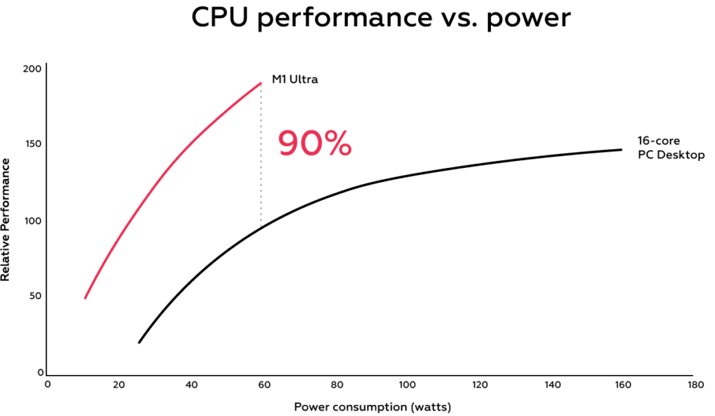
The M1 Ultra CPU has 20 cores and the same number of threads, and is made with 5nm technology. [4][6] In comparison, AMD offers a maximum of 16 cores and 32 threads in 7nm technology [7] (AMD’s new ZEN4 series CPUs are expected to have 5nm technology, but we do not know the exact specifications at this point [3]) and Intel 16 cores and 32 threads in 14nm technology [8]. In view of the above, in theory, the Apple product has a significant advantage over the competition in terms of single thread performance. [Fig. 2]

Performance of the new Apple computer

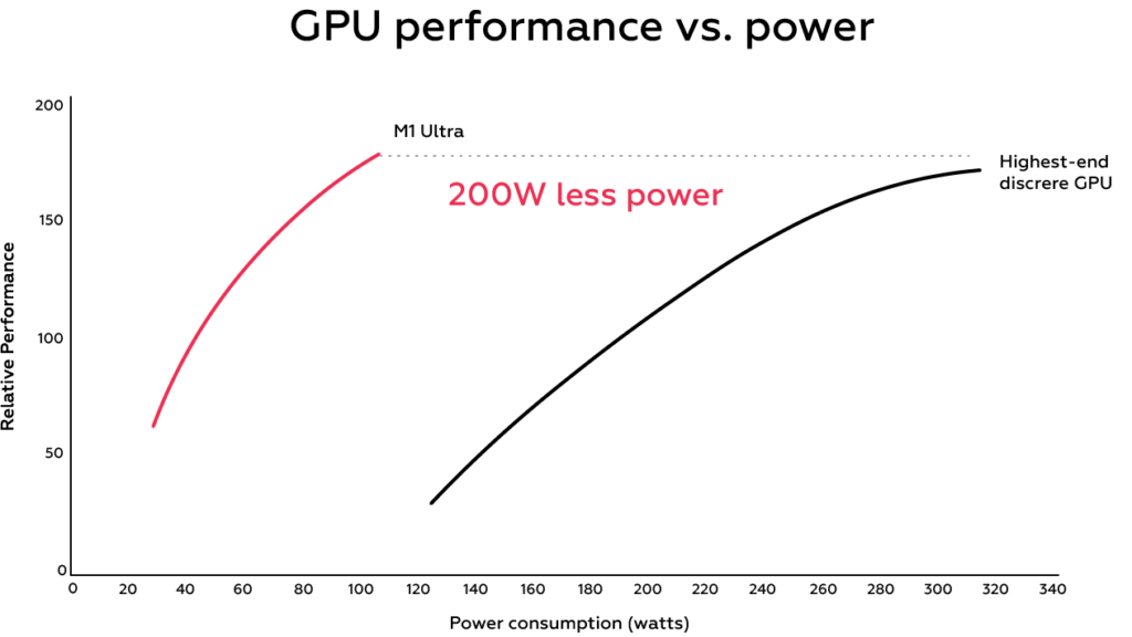
According to the manufacturer’s claims, the GPU from Apple was supposed to outperform the best graphics card available at the time, the RTX 3090.

Graph of the CPU performance against the amount of power consumed
Fig. 2 – Graph of the CPU performance against the amount of power consumed [9]. Graph shown by Apple during the presentation of a new product

The integrated graphics card was supposed to deliver better performance while consuming over 200W less power. [Fig. 3] After the release, however, users quickly checked the manufacturer’s assurances and found that the RTX significantly outperformed Apple’s product in benchmark tests.

Graph of graphics card performance against the amount of power consumed
Fig. 3 – Graph of graphics card performance against the amount of power consumed [9]. Graph shown by Apple during the presentation of a new product. Compared to RTX 3090

The problem is that these benchmarks mostly use software not optimised for the Mac OS, so that the Apple product does not use all of its power. In tests that use the full GPU power, the M1 Ultra performs very similarly to its dedicated rival. Unfortunately, not all applications are written for Apple’s OS, severely limiting the applications in which we will use the full power of the computer.[10]

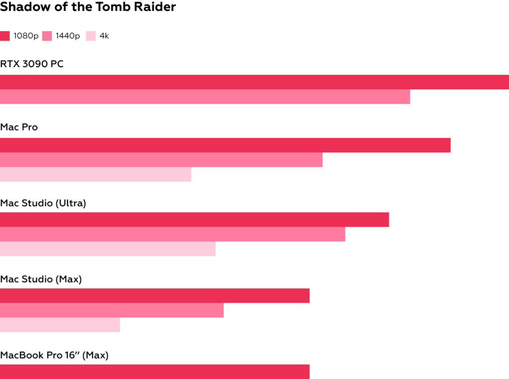
The graph below shows a comparison of the frame rate in “Shadow of the Tomb Raider” from 2018. [Fig. 4] The more frames, the smoother the image.  [2]

The frame rate of the Tomb Raider series game (the more the better)
Fig. 4 – The frame rate of the Tomb Raider series game (the more the better) [2].

Power consumption of the new Mac Studio M1 Ultra compared to standard PCs

Despite its high computer performance, Apple’s new product is very energy-efficient. The manufacturer states that its maximum continuous power consumption is 370W. Standard PCs with modern components do not go below 500W and the recommended power for hardware with the best parts is 1000W [Table 1] ( Nvidia GeForce RTX 3090 Ti + AMD R7/9 or Intel i7/9 ).  

Intel i5
AMD R5
Intel i7
AMD R7
Intel i9 K
AMD R9
NVIDIA RTX 3090 Ti850W1000W1000W
NVIDIA RTX 3090 750W850W850W
NVIDIA RTX 3080 Ti750W850W850W
NVIDIA RTX 3080 750W850W850W
NVIDIA RTX 3070 Ti750W850W850W
NVIDIA RTX 3070 650W750W750W
Lower graphic cards650W650W650W
Table 1 – Table of recommended PSU wattage depending on the CPU and graphics card used. AMD and Intel CPUs in the columns, NVIDIA RTX series graphics cards in the rows. [1]

This means significantly lower maintenance costs for such a computer. Assuming that our computer works 8 hours a day and an average kWh cost of PLN 0.77, we obtain a saving of PLN 1,500 a year. In countries that are not powered by green energy, this also means less pollution.

Apple’s product problems

Products from Apple have dedicated software, which means better compatibility with the hardware and translates into better performance, but it also means that a lot of software not written for Mac OS cannot fully exploit the potential of the M1 Ultra. The product does not allow the use of two operating systems or the independent installation of Windows/Linux. So it turns out that what allows the M1 Ultra to perform so well in some conditions is also the reason why it is unable to compete in performance in other programs. [10]

Conclusion

The Apple M1 Ultra is a powerful computer in a small box. Its 5nm technology provides the best energy efficiency among products currently available on the market. However, due to its low compatibility and high price, it will not replace standard computers. To get maximum performance, dedicated software for the Apple operating system is required. When deciding on this computer, one must keep this in mind. For this reason, despite its many advantages, it is more of a product for professional graphic designers, musicians or video editors.

References

[1] https://www.msi.com/blog/we-suggest-80-plus-gold-1000w-and-above-psus-for-nvidia-geforce-rtx-3090-Ti

[2] https://nano.komputronik.pl/n/apple-m1-ultra/

[3] https://www.tomshardware.com/news/amd-zen-4-ryzen-7000-release-date-specifications-pricing-benchmarks-all-we-know-specs

[4] https://www.x-kom.pl/p/730594-nettop-mini-pc-apple-mac-studio-m1-ultra-128gb-2tb-mac-os.html

[5] https://dailyweb.pl/apple-prezentuje-kosmicznie-wydajny-mac-studio-z-nowym-procesorem-m1-ultra/

[6] https://geex.x-kom.pl/wiadomosci/apple-m1-ultra-specyfikacja-wydajnosc/

[7] https://www.amd.com/pl/partner/ryzen-5000-series-desktop

[8] https://www.cpu-monkey.com/en/

[9] https://www.apple.com/pl/newsroom/2022/03/apple-unveils-m1-ultra-the-worlds-most-powerful-chip-for-a-personal-computer/

[10] https://youtu.be/kVZKWjlquAU?t=301

Sight-playing – part 3

We already created the harmony of the piece in the previous article. What we need now is a good melody which will match this harmony. Melodies consist of motifs, i.e. small fragments of about 2-5 notes and their variations (transformations).

We will start by generating the first motif – its rhythm and sounds. As we did when generating the harmony, we will use N-gram statistics for musical pieces. Such statistics will be prepared using the Essen Folksong Collection base. You might as well use any other melody base, this choice will affect the type of melodies that will be generated. For each piece, we must isolate the melody, convert it into a sequence of rhythmic values and a sequence of sounds, and from these sequences extract the statistics. When compiling sound statistics, it is a good idea to first somehow prepare the melodies – transpose them all to two keys, e.g. C major and c minor. This will reduce the number of possible (probable) N-grams by 12 times and therefore the statistics will be better assessed.

A good motif

We will begin creating the first motif by generating its rhythm. Here, I would like to remind you that we have previously made a certain simplification – each motif and its variations will last exactly one bar. The subsequent steps for generating the rhythm of a motif: – we draw the first rhythmic value using unigrams, – we draw the next rhythmic value using bigrams and unigrams, – we continue to draw consecutive rhythmic values, using N-grams of increasingly higher level (up to 5-grams), – we stop until we reach a total rhythmic value equal to the length of one bar – if we have exceeded the length of 1 bar, we start the whole process from the beginning (such generation is fast enough that we can afford such a sub-optimal trial-and-error method).

The next step is to generate the sounds of the motif. Another simplification we made earlier is that we generate pieces only in C major key, so we will make use of the N-gram statistics created on the basis of pieces transposed to this key, excluding pieces in minor keys. The procedure is similar to that for generating rhythm: – we draw the first sound using unigrams, –we draw the next sound using bigrams and unigrams, – we continue until we have drawn as many sounds as we have previously drawn rhythmic values, – we check whether the motif matches the harmony, if not, we go back and start again – if after approx.

100 attempts we failed to generate a motif matching the harmony, this could mean that with the preset harmony and the preset motif there is a very low probability of drawing sounds that will match the harmony. In this case, we go back and generate a new motif rhythm.

Generate until you succeed

When generating both the motif rhythm and its sounds, we use the trial-and-error method. It will also be used in the generation of motif variations described below. Even if this method may seem “stupid”, it’s simple and it works. Although very often such randomly generated motifs don’t match the harmony, we can afford to make many such mistakes. Even 1000 attempts take a short time to calculate on today’s computers, and this is enough to find the right motif.

Variations with raepetitions

We have the first motif, and now need the rest of the melody. However, we will not continue to generate new motifs, as the piece would become chaotic. We also cannot keep repeating the same motif, as the piece would become too boring. A reasonable solution would be, in addition to repeating the motif, to create a modification of that motif, ensuring variation, but without making the piece chaotic.

There are many methods to create motif variations. One such method is chromatic transposition. It involves transposing all notes upward or downward by the same interval. This method can lead to a situation where a motif variation has sounds from outside the key of the piece. This, in turn, means that the probability that the variation will match the harmony is very low. Another method is diatonic transposition, whereby all notes are transposed by the same number of scale steps. Unlike the previous method, diatonic variations do not have off-key sounds.

Yet another method is to change a single interval; one of the motif intervals is changed, while all other intervals remain unchanged. That way, only one part of the motif (the beginning or the end) is transposed (via chromatic or diatonic transposition). Further methods are to convert two notes with the same rhythmic value to one or to convert one note to two notes with the same rhythmic value. For the first method, if the motif has two notes with the same rhythmic value, its rhythm can be changed by combining these two notes. For the second method, a note is selected at random and converted to two “shorter” notes.

Each of the described methods for creating variations makes it possible to generate different motifs. The listed methods are not the only valid methods; it is possible to come up with many more. The only restriction here is that the generated variation should not differ too much from the original motif. Otherwise, it would constitute a new motif rather than a variation. The border where the variation ends and a different motif begins is conventional in nature.

Etc., etc.

There are many more methods for generating motif variations; it is possible to come up with a lot of these. The only restriction is that the generated variation should not differ too much from the original motif. Otherwise, it would constitute a new motif rather than a variation. The border where the variation ends and another motif begins is rather conventional in nature and everyone “feels”, defines it a little differently.

Is that all?

That would be all when it comes to piece generation. Let us summarise the steps that we have taken:

  1. Generating piece harmony:
    • generating harmonic rhythm,
    • generating chord progression.
  2. Generating melody:
    • generating motif rhythm,
    • generating motif sounds,
    • creating motif variations,
    • creating motifs and variations “until it’s done”, that is, until they match the generated harmony

All that is left is to make sure that the generated pieces are of the given difficulty, i.e. matching the skills of the performer.

Controlling the difficulty

One of our assumptions was the ability to control the piece difficulty. This can be achieved via two approaches:

  1. generating pieces “one after another” and checking their difficulty levels (using the methods described earlier), thereby preparing a large database of pieces from which random pieces of the given difficulty will then be selected,
  2. controlling the parameters for creating the harmonies, motifs and variations in such a way that they generate musical elements of the given difficulty with increased frequency

Both methods are not mutually exclusive and thus can be successfully used together. First, a number of pieces (e.g. 1000) should be generated randomly, and then parameters should be controlled to generate further pieces (but only those which are missing). With respect to parameter control, it is worth noting that the probability of motif repetition can be changed. For pieces with low difficulty, the assigned probability will be higher (repetitions are easier to play). On the other hand, difficult pieces will be assigned lower probability and rarer harmonies (which will also force rarer motifs and variations).

Sight-playing part – 2

In the first part of the article, we have learned about many musical and technical concepts. Now it is time to use them to build an automatic composer.  Before doing so, however, we must make certain assumptions (or rather simplifications):

  • the pieces will consist of 8 bars in periodic structure (antecedent 4 bars, consequent 4 bars)
  • the metre will be 4/4 (i.e. 4 quarter notes to each bar, accent on the first and third measures of the bar)
  • the length of each motif is 1 bar (although this requirement appears restrictive, many popular pieces are built precisely from motifs that last 1 bar).
  • only C major key will be used (if necessary, we can always transpose the piece to any key after its generated)
  • we will limit ourselves to about 25 most common varieties of harmonic degrees (there are 7 degrees, but some of them have several versions, with additional sounds which change the chord colour).

What is needed to create a musical piece?

In order to automatically create a simple musical piece, we need to:

  • generate the harmony of a piece – chords and their rhythm
  • create motifs – their sounds (pitches) and rhythm
  • create variations of these motifs – as above
  • combinate the motifs and variations into a melody, matching them with the harmony

Having mastered the basics, we can move on to the first part of automatic composing – generating a harmony. Let’s start by creating a rhythm of the harmony.

Slow rhythm

Although one might be tempted to create a statistical model of the harmonic rhythm, unfortunately, (at least at the time of writing this article) there is no available base which would make this possible. Given the above, we must handle this in a different way – let’s come up with such a model ourselves. For this purpose, let’s choose a few “sensible” harmonic rhythms and give them some “sensible” probability.

rhythmprobabilityrhythmprobability
[8]0.2[2,2]0.1
[6, 2]0.1[2,1,1]0.02
[2, 6]0.1[3,1]0.02
[7, 1]0.02[1,1,1,1]0.02
[4]0.4[1,1,2]0.02
Table 1. Harmonic rhythms, values expressed in quarter notes – [6, 2] denotes a rhythm in which there are two chords, the first one lasts 6 quarter notes, the second 2 quarter notes.

The rhythms in the table are presented in terms of chord duration, and the duration is shown in the number of quarter notes. Some rhythms last two bars (e.g. [8], [6, 2]), and others one bar ([4], [1, 1, 2] etc.).

Generating a rhythm of the harmony proceeds as follows. We draw new rhythms until we have as many bars as we needed (8 in our case). Sometimes certain complications may arise from the fact that the rhythms have different lengths. For example, there may be a situation where to complete the generation we need the last rhythm that lasts 4 quarter notes, but we draw one that lasts 8 quarter notes. In this case, in order to avoid unnecessary problems, we can force drawing from a subset of 4-quarter-note rhythms.

Then, in line with the above findings, let’s suppose that we drew the following rhythms:

  • antecedent: [4, 4], [2, 2], [3, 1], 
  • consequent: [3, 1], [8], [2, 2]

Likelihood

In the next step, we will be using the concept of likelihood. It is a probability not normalised to one (so-called pseudo-probability), which helps to assess the relative probability level of different events. For example, if the likelihoods of events A and B are 10 and 20 respectively, this means that event B is twice as likely as event A. These likelihoods might as well be 1 and 2 or 0.005 and 0.01. From the likelihoods, probability can be calculated. If we assume that only events A and B can occur, then their probability will be respectively:

Chord progressions

In order to generate probable harmonic flows, we will first prepare the N-gram models of harmonic degrees. To this end, we will use N-gram models available on github (https://github.com/DataStrategist/Musical-chord-progressions).

In our example, we will use 1-, 2-, 3-, 4- and 5-grams.

In the rhythm of the antecedent’s harmony, there are 6 rhythmic values, so we need to prepare the flow of 6 harmonic degrees. We generate the first chord using unigrams (1-grams). Now, we first prepare the likelihoods for each possible degree and then draw while taking these likelihoods into consideration. The formula for likelihood is quite simple in this case

likelihoodX=p(X)

where

  • X means any harmonic degree
  • p(X) is the probability of the 1-gram of X

In this case, we drew IV degree (in this key of F major).

We generate the second chord using bigrams and unigrams, with a greater weight for bigrams.

likelihoodX=weight2gramp(X v IV)+weight1gram*p(X)

where:

  • p(X v IV) is the probability of the flow (IV, X)
  • weightNgram is the adopted N-gram weight (the greater the weight, the greater the impact of this N-gram model, and the smaller the impact of other models)

We can adopt N-gram weights as we wish. For this example, we chose the following:

N-gram12345
weight0.0010.010.115

The next chord we drew was: vi degree (a minor).

The generation of the third chord is similar, except that we can now use 3-grams:

likelihoodX=weight3gramp(X v IV, vi)+weight2gramp(X v IV)+weight1gram*p(X)

And so we continue until we have generated all the necessary chords. In our case, we drew:

IV, vi, I, iii, IV, vi (in the adopted key of C major these are, respectively, F major, a minor, C major, e minor, F major and a minor chords).

This is not a very common chord progression but, as it turns out, it occurs in 5 popular songs (https://www.hooktheory.com/trends#node=4.6.1.3.4.6&key=rel)

Summary

We were able to generate the rhythms and chords which are the components of the harmony of a piece. However, it should still be noted here that, for the sake of simplicity, we didn’t take into account two important factors:

  • The harmonic flows of the antecedent and consequent are very often linked in some way. The harmony of the consequent may be identical with that of the antecedent or perhaps slightly altered to create the impression that these two sentences are somehow linked.
  • The antecedent and consequent almost always end on specific harmonic degrees. This is not a strict rule, but some harmonic degrees are far more likely than others at the end of musical sentences.

For the purposes of the example, however, the task can be deemed completed. The harmony of the piece is ready, now we only need to create a melody to this harmony. In the next part of our article, you will find out how to compose such a melody.

Cloud computing vs environment

The term “cloud computing” is difficult to define in a clear manner. Companies will approach the cloud differently than individuals. Typically, “cloud computing” is used to mean a network of server resources available on demand – computing power and disk space, but also software – provided by external entities, i.e. the so-called cloud providers. The provided resources are accessible via the Internet and managed by the provider, which eliminates the need for companies to purchase hardware and directly manage physical servers. In addition, the cloud is distributed over multiple data centres located in many different regions of the world, which means that users can count on lower failure rates and higher availability of their services [1].

The basic operation of the cloud

Resources available in the cloud are shared by multiple clients, which makes it possible to make better use of the available computing power and, if utilised properly, can prove to be more cost-effective. Such an approach to resource sharing may raise some concerns, but thanks to virtualisation, the cloud provides higher security than the traditional computing model. Virtualisation makes it possible to create simulated computers, so-called virtual machines, which behave like their physical counterparts, but reside on a single server and are completely isolated from each other. Resource sharing and virtualisation allow for efficient use of hardware and ultimately reduce power consumption by server rooms. Financial savings can be felt thanks to the “pay-as-you-go” business model commonly used by providers, which means that users are billed for actually used resources (e.g. minutes or even seconds of used computing time), as opposed to paying a fixed fee. 

The term “cloud” itself originated as a slang term. In technical diagrams, network and server infrastructure is often represented by a cloud icon [2]. Currently, “cloud computing” is a generally accepted term in IT and a popular computing model. The affordability of the cloud and the fact that users are not required to manage it themselves mean that this computing model is being increasingly preferred by IT companies, which has a positive impact on environmental aspects [3].

Lower power consumption 

The increasing demand for IT solutions leads to increased demand for electricity – a strategic resource in terms of maintaining the cloud. A company maintaining its own server room leads to significant energy expenditure, generated not only by the computer hardware itself but also by the server room cooling system. 

Although it may seem otherwise, larger server rooms which process huge amounts of data at once are more environmentally friendly than local server rooms operated by companies [4]. According to a study carried out by Accenture, migrating a company to the cloud can reduce power consumption by as much as 65%. This stems from the fact that cloud solutions on the largest scale are typically built at dedicated sites, which improves infrastructure organisation and resource management [5]. Providers of large-scale cloud services can design the most effective cooling system in advance. In addition, they make use of modern hardware, which is often much more energy-efficient than the hardware used in an average server room. A study conducted in 2019 revealed that the AWS cloud was 3.6 times more efficient in terms of energy consumption than the median of the surveyed data centres operated by companies in the USA [6].

Moreover, as the cloud is a shared environment, performance can be effectively controlled. The scale of the number of users of a single computing cloud allows for a more prudent distribution of consumed energy between individual cases. Sustainable resource management is also enabled by our Data Engineering product, which collects and analyses data in order to maximise operational efficiency and effectiveness.

Reduction of emissions of harmful substances

Building data processing centres which make use of green energy sources and are based on low-emission solutions makes it possible, among others, to control emissions of carbon dioxide and other gases which contribute to the greenhouse effect. According to data presented in the “The Green Behind Cloud” report [7], migrating to public cloud can reduce global carbon dioxide emissions by 59 million tonnes per year, which is equivalent to removal of 22 million cars from the roads.

It is also worth considering migration to providers which are mindful of their carbon footprint. For example, the cloud operated by Google is fully carbon-neutral through the use of renewable energy, and the company promises to use only zero-emission energy around the clock in all data centres by 2030 [8]. The Azure cloud operated by Microsoft has been carbon-neutral since 2012, and its customers can track the emissions generated by their services using a special calculator [9].

Reduction of noise related to the use of IT hardware  

Noise is classified as environmental pollution. Though at first glance it may appear quite inconspicuous and harmless, it has a negative impact on human health and the quality of the environment. With respect to humans, it increases the risk of such diseases as cancer, myocardial infarction and arterial hypertension. With respect to the environment, it leads to changes in animal behaviour and affects bird migration and reproduction.

The main source of noise in solutions for storing data on company servers is a special cooling system which maintains the appropriate temperature in the server room. Using cloud solutions makes it possible to reduce the noise emitted by cooling devices at workplaces, which helps limit environmental noise pollution.

If you want to learn more about the available solutions for reducing industrial noise, check our Intelligent Acoustics product.

Waste level reduction 

Making use of cloud computing in business activities, as opposed to having traditional servers as part of company resources, also helps reduce the amount of generated electronic waste. This stems primarily from the fact that cloud computing does not necessitate the purchase of additional equipment or preparation of infrastructure for a server room at the company, which reduces the amount of equipment that needs to be disposed of in the long term.  

In addition, the employed virtualisation mechanisms, which entail the replacement of a larger number of low-performance servers with a smaller number of high-performance servers which are able to use this performance more effectively, optimise and increase server efficiency, and thus reduce the demand for hardware resources.  

Summary 

Sustainability is currently an important factor in determining the choice of technology. Environmental protection is becoming a priority for companies and for manufacturers of network and telecommunications devices, which means that greener solutions are being sought. Cloud computing definitely fits this trend. It not only limits the consumption of hardware and energy resources, but also reduces the emission of harmful substances into the ecosystem as well as noise emissions into the environment.  

References 

[1] https://www.wit.edu.pl/dokumenty/wydawnictwa_naukowe/zeszyty_naukowe_WITZ_06/0006_Joszczuk-Januszewska.pdf 

[2] https://rocznikikae.sgh.waw.pl/p/roczniki_kae_z36_21.pdf 

[3] http://yadda.icm.edu.pl/yadda/element/bwmeta1.element.ekon-element-000171363539  

[4] Paula Bajdor, Damian Dziembek “Środowiskowe i społeczne efekty zastosowania chmury obliczeniowej w przedsiębiorstwach” [“Environmental and Social Effects of the Use of Cloud Computing in Companies”], 2018 

[5] https://www.accenture.com/_acnmedia/PDF-135/Accenture-Strategy-Green-Behind-Cloud-POV.pdf  

[6] “Reducing carbon by moving to AWS” https://www.aboutamazon.com/news/sustainability/reducing-carbon-by-moving-to-aws

[7] https://www.accenture.com/us-en/insights/strategy/green-behind-cloud

[8] “Operating on 24/7 Carbon-Free Energy by 2030.” https://sustainability.google/progress/energy/

[9] https://www.microsoft.com/en-us/sustainability/emissions-impact-dashboard

ANC — Financial Aspects

Today’s realities are making people increasingly inclined to discuss finances. This applies to both private household budgets and major, global-level investment projects. There is no denying the fact that attention to finances has resulted in the development of innovative methods of analysing them. These range from simple applications that allow us to monitor our day-to-day expenses to huge accounting and bookkeeping systems that support global corporations. The discussions about money also pertain to investment projects in a broader sense. They are very often associated with the implementation of modern technologies, which are implicitly intended to bring even greater benefits, with the final result being greater profit. Yet how do you define profit? And is it really the most crucial factor in today’s perception of business? Finally, how can active noise reduction affect productivity and profit?

What is profit?

The literature explains that “profit is the excess of revenue over costs” [1]. In other words, profit is a positive financial result. Colloquially speaking, it is a state in which you sell more than you spend. This is certainly a desirable phenomenon since, after all, the idea is for a company to be profitable. Profit serves as the basis for further investment projects, enabling the company to continue to meet customer needs. Speaking of profit, one can distinguish several types of it [2]:

  1. Gross profit, i.e. the difference between net sales revenue and costs of products sold. It allows you to see how a unit of your product translates into the bottom line. This is particularly vital for manufacturing companies, which often seek improvements that will ultimately allow them to maintain economies of scale.
  2. Net profit, i.e. the surplus that remains once all costs have been deducted. In balance sheet terms, this is the difference between total costs and sales revenue. In today’s world, it is frequently construed as a factor that indicates the financial health of an enterprise.
  3. Operating profit, i.e. a specific type of profit that is focused solely on the company’s result in its core business area. It is very often listed as EBIT in the profit and loss account.

Profit vs productivity

In this sense, productivity involves ensuring that the work does not harm the workers’ lives or health over the long term. The general classification of the Central Institute for Labour Protection lists such harmful factors as [3]:

  • noise and mechanical vibration,
  • mechanical factors,
  • chemical agents and dust,
  • musculoskeletal stress,
  • stress,
  • lighting,
  • optical radiation,
  • electricity.

The classification also lists thermal loads, electromagnetic fields, biological agents and explosion and fire hazards. Yet the most common problem is that of industrial noise and vibrations that the human ear is often unable to pick up at all. It has often been the case that concentration decreased while sleepiness levels increased while working in a perpetually noisy environment. Hence, one may conclude that even something as inconspicuous as noise and vibration generates considerable costs for the entrepreneur, especially in terms of unit costs (for mass production). As such, it is crucial to take action in noise reduction. If you would like to learn more about how to combat noise pollution, click here to sign up for training.

How do you avoid incurring costs?

Today’s R&D companies, engineers and specialists thoroughly research and improve production systems, which allows them to develop solutions that eliminate even the most intractable human performance problems. Awareness of better employee care is deepening year on year. Hence the artificial intelligence boom, which is aimed at creating solutions and systems that facilitate human work. However, such solutions require a considerable investment, and as such, financial engineers make every effort to optimise their costs.

Step 1 — Familiarise yourself with the performance characteristics of the factory’s production system in production and economic terms.

Each production process has unique performance and characteristics, which affect production results to some extent. To be measurable, these processes must be examined using dedicated indicators beforehand. It is worth determining process performance at the production and economic levels based on the knowledge of the process and the data that is determined using such indicators. The production performance determines the level of productivity of the human-machine team, while the economic performance examines the productivity issue from a profit or loss perspective. Production bottlenecks that determine process efficiency are often identified at this stage. It is worthwhile to report on the status of production efficiency at this point.

Step 2 — Determine the technical and economic assumptions

The process performance characteristics report serves as the basis for setting the assumptions. It allows you to identify the least and most efficient processes. The identification of assumptions is intended to draw up current objectives for managers of specific processes. In the technical dimension, the assumptions typically relate to the optimisation of production bottlenecks. In the economic dimension, it is worth focusing your attention on cost optimisation, resulting from the cost accounting in management accounting. Technical and economic assumptions serve as the basis for implementing innovative solutions. They make it possible to greenlight the changes that need to happen to make a process viable.

Step 3 — Revenue and capital expenditure forecasts vs. active noise reduction

Afterwards, you must carry out predictive testing. It aims to examine the distribution over time of the revenue and capital expenditure incurred for both the implementation and subsequent operation of the system in an industrial setting.

Forecasted expenditure with ANC
Figure 1 Forecast expenditure in the 2017-2027 period
Forecasted revenue with ANC
Figure 2 Forecast revenue in the 2017-2027 period

From an economic standpoint, the implementation of an active noise reduction system can calm income fluctuations over time. The trend based on the analysis of the previous periods clearly shows cyclicality and a linear trend in terms of both increases and decreases. Stabilisation correlates with the implementation of the system described. This may involve a permanent additional increase in the capacity associated with the system’s implementation into the production process. Hence the conclusion that improvements in productive efficiency result in income stabilisation over time. On the other hand, the implementation of the system requires higher expenditures. The expenditure level is trending downwards year on year, however.

This data allows you to calculate basic measures of investment profitability. At this point, you can also carry out introductory calculations to determine income and expenditure at a single point in time. This allows you to calculate the discount rate and forecast future investment periods [1].

Step 4 — Evaluating investment project effectiveness using static methods

Calculating measures of investment profitability allows you to see if what you wish to put your capital into will give you adequate and satisfactory returns. When facing significant competition, investing in such solutions is a must. Of course, the decisions taken can tip the balance in two ways. Among the many positive aspects of investing are increased profits, reduced costs and a stronger market position. Yet there is also the other side of the coin. Bad decisions, typically based on ill-prepared analyses or made with no analyses at all, often involve lost profits and may force you to incur opportunity costs as well. Even more often, ill-considered investment projects result in a decline in the company’s value. In static terms, we are talking about the following indicators:

  • Annual rate of return,
  • Accounting rate of return,
  • Payback period.

In the present case, i.e. the implementation of an active noise reduction system, we are talking about an annual and accounting rate of return of approximately 200% of the value. The payback period settles at less than a year. This is due to the large disparity between the expenses incurred in implementing the system and the benefits of its implementation. However, to be completely sure of implementation, the Net Present Value (NPV) and Internal Rate of Return (IRR) still need to be calculated in the first place. The NPV and IRR determine the performance of the investment project over the subsequent periods studied.

Step 5 — Evaluating effectiveness using dynamic methods

In this section, you must consider the investment project’s efficiency and the impact that this efficiency has on its future value. Therefore, the following indicators must be calculated:

  • Net Present Value (NPV),
  • Net Present Value Ratio (NPVR),
  • Internal Rate of Return (IRR),

In pursuing a policy of introducing innovation in industrial companies, companies face the challenge of maximising performance indicators. Considering the correlation between the possibilities of applying active noise reduction methods that improve the working conditions, thus influencing employee performance, one may conclude that the improvement in work productivity is reflected in the financial results, which has a direct impact on the assessment of the effectiveness of such a project. Despite the high initial expenditures, this solution offers long-term benefits by improving production stability.

Is it worth carrying out initial calculations of investment returns?

To put it briefly: yes, it is. They prove helpful in decision-making processes. They represent an initial screening for decision-makers — a pre-selection of profitable and unprofitable investment projects. At that point, the management is able to establish the projected profitability even down to the operational level of the business. Reacting to productivity losses allows bosses to identify escaping revenue streams and react earlier to potential technological innovations. A preliminary assessment of cost-effectiveness is a helpful tool for making accurate and objective decisions.

References

[1] D.Begg, G.Vernasca, S.Fischer „Mikroekonomia” PWE Warszawa 2011
[2] mfiles.pl/pl/index.php/Zysk

[3] Felis P., 2005: Metody i procedury oceny efektywności inwestycji rzeczowych przedsiębiorstw. Wydawnictwo Wyższej Szkoły Ekonomiczno-Informatycznej. Warszawa.

Digital image processing

Signal processing accompanies us every day. All stimuli (signals) received from the world around sound, light, or temperature are processed into electrical signals, which are later sent to the brain. In the brain, the analysis and interpretation of the received signal takes place. As a result, we get information from the signal (e.g. we can recognize the shape of an object, we feel the heat, etc.).

Digital signal processing (DSP) works similarly. In this case, the analog signal is converted into a digital signal by an analog-digital converter. Then, using the digital computer, received signals are being processed. The DSP systems also use computer peripheral devices equipped with signal processors which allow processing of signals in real-time. Sometimes, it is necessary to re-convert the signal to an analog form (e.g. to control a device). For this purpose, digital-to-analog converters are used.

Digital signal processing has a wide range of applications. It can be used to process sound, speech recognition, or image processing. The last issue will be the subject of this article. We will deeply discuss the basic operation of convolutional filtration in digital image processing.

What is image processing?

Simply speaking, digital image processing consists in transforming the input image into an output image. The aim of this process is to select information – choosing the most important (e.g. shape) and eliminating unnecessary (e.g. noise). The digital image process features a variety of different image operations such as:

  • filtration,
  • thresholding,
  • segmentation,
  • geometry transformation,
  • coding,
  • compression.

  As we mentioned before, in this article we will focus on image filtration.

Convolutional filtration

Both in the one-dimensional domain (for audio signals) and also for two dimensions, there are specific tools for operating on signals – in this case on images. One of such tools is filtration. It consists of some mathematical operations on pixels which as a result give us a new image. Filtration is commonly used to improve image quality or to extract important features from the image.

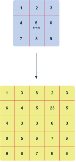
The basic operation in the filtration method is the 2D convolutional function. It allows applying of image transformations using appropriate filters in a form of matrix coefficients. The use of filters consists of calculating a point’s new value based on the brightness values of points in the closest neighborhood. Such so-called masks containing pixel weights based on the closest pixels values are used in calculations. The usual sizes of masks are 3×3, 5×5, and 7×7. The process of image and filter convolution has been shown below.

Assuming that the image is represented by a 5×5 matrix which contains color values and the filter is represented by a 3×3 matrix, the image was modified by joining these matrices.

The first thing to do is to transpose coefficients in a filter. We assume that the center of the filtration core h(0,0) is in the middle of the matrix, as shown in the picture below. Therefore (m,n) indexes denoting rows and columns of the filter matrix will be both negative and positive.

Image filtration diagram
Img 1 Filtration diagram

Considering the filter matrix (the blue one) as inverted vertically and horizontally we can perform filtration operations. They start by placing the h(0,0) → h(m,n) element of the blue matrix over the s(-2,-2) → s(i,j) element of the yellow matrix (the image). Then we multiply the overlapping values of both matrices and add them up. In this way, we have obtained the convolution result for the (-2,-2) cell of the output image. It is important to remember the normalization process, which allows us to adjust the brightness of a result by dividing it by the sum of filter coefficients. It prevents the output image brightness from being out of a scale of 0-255 (in the case of 8-bit image representation).

The next stages of this process are very similar. We move the center of the blue matrix over the (-2,-1) cell, then again multiply the overlapping values. Next, add them together and divide the result by the filter coefficients to get the result. We consider cells that go beyond the area of the matrix s (i,j) to be undefined. Therefore, the values do not exist in these places, so we do not multiply them.

The usage of convolutional filtration

Depending on the type of filter, we can distinguish several applications of convolutional filtration. Low-pass filters are used to remove noise from images, while high-pass filters are used to sharpen or emphasize edges. To illustrate the effects of different filters, we will apply them to the real image. The picture below is a “jpg” format and was loaded in Octave software as an MxNx3 pixel matrix.

Original input image
Img 2 Original Input Image

Gaussian blur

To blur the image we need to use a convolutional function as well as the properly prepared filter. One of the most commonly used low-pass filters is the gaussian filter. It allows you to lower the sharpness of the image but also it is used to reduce the noise from it.

For this article, a 29×29 matrix based on Gaussian function with a standard deviation of 5 was generated. The normal distribution gives weights to the surrounding pixels during the process of convolution. A low-pass filter suppresses high-frequency image elements while passing low-frequency elements. The output image compared to the original one is blurry, and the noises are significantly reduced.

Blurred input image
Img 3 Blurred input image

Sharpen

We can make the image blurry but there is also a way to make it sharpen. To make it happen a suitable high-pass filter should be used. The filter passes through and amplifies image elements that are characterized by high frequency e.g. noise or edges. However, low-frequency elements are suppressed. By using this filter, the original image is sharpened – it can be easily noticed especially in the arm area.

Sharpened input image
Img 4 Sharpened input image

Edges detection

Another possible image process is called edge detection. Shifting and subtracting filters are used to detect edges on the image. They work by shifting the image and subtracting the original image from its copy. As a result of this procedure, edges are being detected, as shown in the picture below.

Edge detection
Img 5 Edge detection

BFirst.Tech experience with image processing

Our company hires well-qualified staff with experience in the field of image processing. One of our original projects was called TIRS, i.e. a platform which diagnoses areas in the human body that might be affected by cancerous cells. It works based on the use of advanced image processing algorithms and artificial intelligence. It automatically detect cancerous areas with the use of medical imaging data obtained from tomography and magnetic resonance imaging. This platform finds its use in clinics and hospitals.

Our other project, which also requires the usage of image processing, is called the Virdiamed platform. It was created in cooperation with Rehasport Clinic. This platform allows a 3D reconstruction of CT and MRI data and also allows the viewing of 3D data in a web browser. If you want to read more about our projects, click here.

Digital signal processing, including image processing, is a field of technology with a wide range of application possibilities, and its popularity is constantly growing.  Non-stopping technological progress means that this field of technology is also constantly developing. Moreover, any technologies used every day are based on signal processing, which is why it is certain that in the future the importance of DSP will continue to grow.

References

[1] Leonowicz Z.: „Praktyczna realizacja systemów DSP”

[2] http://www.algorytm.org/przetwarzanie-obrazow/filtrowanie-obrazow.html

Smart Manufacturing

New technologies are finding their place in many areas of life. One of these is an industry, where advanced technologies have been used for years and work very well for factories. The implementation of smart solutions based on advanced IT technologies into manufacturing companies has had a significant impact on technological development and improved innovation. One of them is Smart Manufacturing, which helps industrial optimisation by drawing insights from data generated in manufacturing processes.

What is meant by Smart Manufacturing?

Smart Manufacturing is a concept that encompasses the full integration of systems with collaborative production units that are able to react in real time and adapt to changing environmental conditions, making it possible to meet the requirements within the supply chain. The implementation of an intelligent manufacturing system supports the optimisation of production processes. At the same time, it contributes to increased profits for industrial companies.

The concept of Smart Manufacturing is closely related to concepts such as artificial intelligence (AI), the Industrial Internet of Things (IIoT) or cloud computing. What these three concepts have in common is data. The idea behind smart manufacturing is that the information it contains is available whenever necessary and in its most useful form. It is data analysis that has the greatest impact on optimising manufacturing processes and makes them more efficient.

IIoT and industrial optimisation

The Industrial Internet of Things is nothing more than the application of IoT potential in the industrial sector. In the intelligent manufacturing model, people, machines and processes are interconnected through IT systems. Each machine features sensors that collect vital data about its operation. The system sends the data to the cloud, where it goes through and extensive analysis. With the information obtained from them, employees have an insight into the exact process flow. Thanks to that, they are able to anticipate failures and prevent them earlier, avoiding possible downtime. In addition, companies can examine trends in the data or run various simulations based on the data. The integration of all elements of the production process also makes it possible to remotely monitor its progress in real time, as well as to react to any irregularities. All of that would not be possible if it wasn’t for the IIoT solutions.

The rise of artificial intelligence

Another modern technological solution that is used in the smart manufacturing system is artificial intelligence. Over the last few years, we have seen a significant increase in the implementation of artificial intelligence solutions in manufacturing. This is now possible, precisely because of the deployment of IIoT devices, which provide huge amounts of data used by AI. Artificial intelligence algorithms analyse the data obtained and search for anomalies in the data. In addition, they enable automated decision-making based on the collected data. What’s more, artificial intelligence is able to predict problems before they occur and take appropriate steps to mitigate them.

Benefits for an enterprise

The implementation of Smart Manufacturing technology in factories can bring a number of benefits, primarily in the optimisation of manufacturing processes. With smart manufacturing, the efficiency can be improved tremendously. By having access to data on the entire process, it is possible to react quickly to any potential irregularities or adapt the process to current needs (greater flexibility). This allows companies to avoid many unwanted events, like breakdowns. This, in turn, has a positive effect on cost optimisation while also improving the company’s profitability. Yet another advantage is better use of machinery and equipment. By monitoring them on an ongoing basis, companies can control their wear and tear, anticipate breakdowns or plan downtime in a more efficient manner. This, in turn, improves productivity and even the quality of the manufactured products.

The use of SM also enables real-time data visualisation. That makes it possible to manage – as well as monitor – the process remotely. In addition, the virtual representation of the process provides an abundance of contextual information that is essential for process improvement. Based on the collected data, companies can also run various types of simulations. They can also anticipate trends or potential problems, which greatly improves forecasting. We should also mention here that implementing modern solutions such as Smart Manufacturing in a company increases their innovativeness. Thus, companies become more competitive and employees perceive them as a more attractive place to work.

Will automation put people out of work?

With technological developments and the increasingly widespread process automation, concerns regarding losing jobs have also become more apparent. Nothing could be further from the truth – people still play a pivotal role in the concept of smart manufacturing. The responsibility of employees to control processes or make critical decisions will therefore remain unchanged. Human-machine collaboration will thus make it possible to increase the operational efficiency of the smart enterprise.

So – the intention behind technological development is not to eliminate man, but rather to support him. What’s more, the combination of human experience and creativity with the ever-increasing capabilities of machines makes it possible to execute innovative ideas that can have a real impact on improving production efficiency. At the same time, the labour market will start to see an increased demand for new experts, ensuring that the manufacturing industry will not stop hiring people.

Intelligent manufacturing is an integral part of the fourth industrial revolution that is unfolding right before our eyes. The combination of machinery and IT systems has opened up new opportunities for industrial optimisation. This allows companies to realistically increase the efficiency of their processes, thereby helping to improve their profitability. BFirst.Tech offers an Industrial Optimisation service to analyse and communicate real-time data to all stakeholders with the contained information supporting critical decision-making and results in continuous process improvement.

References

[1] https://blog.marketresearch.com/the-top-7-things-to-know-about-smart-manufacturing

[2] https://przemyslprzyszlosci.gov.pl/7-krokow-do-zaawansowanej-produkcji-w-fabryce-przyszlosci/?gclid=EAIaIQobChMIl7rb1dnD7QIVFbd3Ch21kwojEAAYASAAEgKVcfD_BwE

[3] https://www.comarch.pl/erp/nowoczesne-zarzadzanie/numery-archiwalne/inteligentna-produkcja-jutra-zaczyna-sie-juz-dzis/

[4] https://elektrotechnikautomatyk.pl/artykuly/smart-factory-czyli-fabryka-przyszlosci

[5] https://www.thalesgroup.com/en/markets/digital-identity-and-security/iot/inspired/smart-manufacturing

[6] https://www.techtarget.com/iotagenda/definition/smart-manufacturing-SM

Data Warehouse

A data warehouse is one of the more common topics in the IT industry. The collected data is an important source of valuable information for many companies, thus increasing their competitive advantage. More and more companies use Business Intelligence (BI) systems in their work, which quickly and easily support the analytical process. BI systems are based on data warehouses and we will talk about them in today’s article.

What is a data warehouse?

A data warehouse is one of the more common topics in the IT industry. The collected data is an important source of valuable information for many companies, thus increasing their competitive advantage. More and more companies use Business Intelligence (BI) systems in their work, which quickly and easily support the analytical process. BI systems are based on data warehouses and we will talk about them in today’s article.

Characteristics

There are four main features that characterize a data warehouse. These are:

  • Subject orientation – the collected data is organized around main topics such as sales, product, or customer;
  • Integrity – the stored data is uniform, e.g. in terms of format, nomenclature, and coding structures. They are standardized before they reach the warehouse;
  • Timeliness – the data comes from different time frames, it contains both historical and current data;
  • Non-volatile – the data in the warehouse remains unchanged. The user cannot modify it, so we can be sure that we will get the same results every time.

Architecture and operation

In the architecture of a data warehouse, four basic components can be distinguished. Data sources, ETL software, the appropriate data warehouse, and analytical applications. The following graphic shows a simplified diagram of that structure.

Data warehouse graph
Img 1 Diagram of data warehouse operation

As can be seen from the graphic above, the basis for building each data warehousing system is data. The sources of this data are dispersed – they include ERP, CRM, SCM, or Internet sources (e.g. statistical data).

The downloaded data is processed and integrated and then loaded into a proper data warehouse. This stage is called the ETL process, from the words: extract, transform and load. According to the individual stages of the process, data is first taken from available sources (extract). In the next step, the data is transformed, i.e. processed in an appropriate way (cleaning, filtering, validation, or deleting duplicate data). The last step is to load the data to the target database, i.e. the data warehouse.

As we mentioned earlier, the data collected is read-only. Users call data from the data warehouse using appropriate queries. On this account, obtaining data is presented in a more friendly form, i.e. reports, diagrams, or visualizations.

Main tasks

As the main task of a data warehouse, analytical data processing (OLAP, On-Line Analytical Processing) should be distinguished. It allows for making various types of summaries, reports, or charts presenting significant amounts of data. For example, a sales chart in the first quarter of the year, a report of products generating the highest revenue, etc.

The next task of that tool is decision support in enterprises (DSS, Decision Support System). Taking into account the huge amount of information that is in the data warehouses, they are a part of the decision support system for companies. Thanks to advanced analyses conducted with the use of these databases, it is much easier to search for dominant trends, models, or relations between various factors, which may facilitate managerial decision-making.

Another of the tasks of these specific databases is to centralize data in the company. Data from different departments/levels of the company are collected in one place. Thanks to that, everyone interested has access to them whenever he or she needs them.

Centralization is connected with another role of a data warehouse, which is archiving. Because the data collected in the warehouse comes from different periods and the warehouse is supplied with new, current data on an ongoing basis, it also becomes an archive of data and information about the company.

Summary

Data warehousing is undoubtedly a useful and functional tool that brings many benefits to companies. Implementation of this database in your company may facilitate and speed up some of the processes taking place in companies. An enormous amount of data and information is generated every day. Therefore, data warehouses are a perfect answer to store this information in one, safe place, accessible to every employee. If you want to introduce a data warehousing system to your company, check our product Data Engineering.

Bibliography

[1] https://www.oracle.com/pl/database/what-is-a-data-warehouse/

Technology trends for 2021

For many people, 2020 will remain a memory they are not likely to quickly forget. The coronavirus pandemic has, in a short time, caused many companies to change their previous way of operating, adapting to the prevailing conditions. The issue of employee safety has become crucial, hence many companies have decided to turn to remote working mode. There is no denying that this situation has accelerated the digital transformation process in many industries, thus contributing to the faster development of modern technologies.

As they do every year, the major analyst firms publish rankings in which they present their new technology predictions for the coming year.

Internet of Behaviours

The concept of the Internet of Behaviour (IoB) emerged some time ago, but, according current for forecasts, we are going to see significant growth in 2021 and beyond. It involves collecting data about users and linking it to specific types of behaviour. The aim is to improve the process of customer profiling and thus consciously influence their behaviour and decisions they make. IoB employs many different modern technologies – from AI to facial or speech recognition. When it comes to IoB, the safety of the collected data is definitely a moot point. On top of that there are ethical and social aspects of using this data to influence consumers.

Cybersecurity

Because of the COVID-19 pandemic lot of companies now operate in remote working mode. Therefore, the question of cyber security has now become more important than ever. Currently, this is a key element in ensuring the safe operation of the organisation. With the popularisation of remote working, cyber threats have also increased. It is, therefore, anticipated that companies will invest in strengthening their security systems to make sure that their data is protected and to prevent possible cyber-attacks.

Anywhere operations

Anywhere operations model is the biggest technology trend of 2021. It is about creating an IT environment that will give people the opportunity to work from just about anywhere by implementing business solutions based on a distributed infrastructure. This type of solution will allow employees to access the organisation’s resources regardless of where they are working and facilitate the exchange and flow of information between them. According to Gartner’s forecasts, as much as 40% of organisations will have implemented this operating model in their organisation by 2023.

AI development

The list the biggest modern technologies trends of 2021 would not be complete without artificial intelligence, the steady development of which we’re constantly experiencing. AI solutions such as forecasting, speech recognition or diagnostics are used in many different industries. Machine learning models are also increasingly popular in factories, helping to increase the efficiency of their processes. Over the next few years, we will see the continued development of artificial intelligence, and the exploitation of the potential it holds.

Total Experience

Another trend that will most likely be big this year is Total Experience (TX), which is intended to bring together the differing perspectives of customers, employees and users to improve their experience where these elements become intertwined. This approach combined with modern technology is supposed to give some companies competitive edge. As a result of the pandemic most of the interactions among the aforementioned groups happens online. This is why it is so important for their respective experiences to bring them certain kind of satisfaction, which will have an actual impact on the companies’ performance.

This year’s technology trends mainly focus on the development of solutions aimed at improving remote working and the experience of moving much of our lives to the online sphere. There is no denying that the pandemic has significantly accelerated the technological development of many companies. This rings particularly true for the micro-enterprises that have had to adapt to the prevailing conditions and have undergone a digital transformation. An important aspect among the projected trends is undeniably providing cyber security, both for organisations and individuals. BFirst.Tech seeks to adapt to the growing demand for these issues, which is why it offers a Cloud and Blockchain service that employs modern technology to create secure data environments.

References

[1] https://www.gartner.com/en/newsroom/press-releases/2020-10-19-gartner-identifies-the-top-strategic-technology-trends-for-2021

[2] https://mitsmr.pl/b/trendy-technologiczne-2021/PQu9q8s0G

[3]https://www.magazynprzemyslowy.pl/artykuly/7-trendow-w-it-na-2021-rok

[4] https://www.nbc.com.pl/trendy-technologiczne-w-2021%E2%80%AFroku/

Sight-playing — part 1

During their education, musicians need to acquire the ability to play a vista, that is, to play an unfamiliar piece of music without having a chance to get familiar with it beforehand. Thanks to this, virtuosos can not only play most pieces without preparation but also need much less time to learn the more demanding ones. However, it takes many a musical piece for one to learn how to play a vista. The pieces used for such practice should be little-known and matched to the skill level of the musician concerned. Therefore, future virtuosos must devote a lot of their time (and that of their teachers) to preparing such a playlist, which further discourages learning. Worse still, once used, a playlist is no longer useful for anything.

The transistor composer

But what if we had something that could prepare such musical pieces on its own, in a fully automated way? Something that could not only create the playlist but also match the difficulty of the musical pieces to the musician’s skill level. This idea paved the way for the creation of an automatic composer — a computer programme that composes musical pieces using artificial intelligence, which has been gaining popularity in recent times.

Admittedly, the word “composing” is perhaps somewhat of an exaggeration and the term “generating” would be more appropriate. Though, after all, composers create musical pieces based on their own algorithms. Semantics aside, what matters here is that such a (simple, for the time being) programme has been successfully created and budding musicians could benefit from it.

However, before we discuss how to generate musical pieces, let us first learn the basics of how musical pieces are structured and what determines their difficulty.

Fundamentals of music

The basic concepts in music include the interval, semitone, chord, bar, metre, musical scale and key of a musical piece. An interval is a quantity that describes the distance between two consecutive notes of a melody. Although its unit is the semitone, it is common practice to use the names of specific intervals. In contrast, a semitone is the smallest accepted difference between pitches (approximately 5%). While these differences can be infinitely small, it is simply that this division of intervals has become accepted as standard. A chord is three or more notes played simultaneously. The next concept is the bar, which is what lies between the vertical dashes on the stave. Sometimes a musical piece may begin with an incomplete bar (anacrusis).

Visualization of the anacrusis
Figure 1 Visualisation of an anacrusis

Metre — this term refers to how many rhythmic values are in one bar. In 4/4 metre, there should be four quarter notes to each bar. In 3/4 metre, there should be three quarter notes to each bar while 6/8 metre should have six eighth notes to each bar. Although 3/4 and 6/8 denote the same number of rhythmic values, these metres are different, the accents in them falling on different places in the bar. In 3/4 metre, the accent falls on the first quarter note (to put it correctly, “on the downbeat”). By comparison, in 6/8 metre, the accent falls on the first and fourth measures of the bar.

A musical scale is a set of sounds that define the sound material that musical works use. The scales are ordered appropriately — usually by increasing pitch. The most popular scales are major and minor. While many more scales exist, these two predominate in the Western cultural circle. They were used in most of the older and currently popular pieces. Another concept is key, which identifies the tones that musical pieces use. In terms of scale vs. key, scale is a broader term; there are many keys of a given scale, but each key has its own scale. The key determines the sound that the scale starts with.

Structure of a musical piece

In classical music, the most popular principle for shaping a piece of music is periodic structure. The compositions are built using certain elements, i.e. periods, which form a separate whole. However, several other concepts must be introduced to explain them.

motif is a sequence of several notes, repeated in the same or slightly altered form (variation) elsewhere in the work. Typically, the duration of a motif is equal to the length of one bar.

variation of a motif is a form of the motif that has been altered in some way but retains most of its characteristics, such as rhythm or a characteristic interval. musical pieces do not contain numerous motifs at once. A single piece is mostly composed of variations of a single motif. Thanks to this, each musical piece has a character of its own and does not surprise the listener with new musical material every now and then.

A musical theme is usually a sequence of 2-3 motifs that are repeated (possibly in slightly altered versions) throughout the piece. Not every piece of music needs to have a theme.

A sentence is two or more phrases.

A period is defined by the combination of two musical sentences. Below is a simple small period with its basic elements highlighted.

Scheme of the periodic structure of a musical piece
Figure 2 Periodic structure diagram of a musical piece

This is roughly what the periodic structure looks like. Several notes form a motif, a few motifs create a phrase, a few phrases comprise a sentence, a few sentences make up a period, and finally, one or more periods form a whole musical piece. There are also alternative methods of creating musical pieces. However, the periodic structure is the most common, and importantly in this case, easier to program.

Composing in harmony

Compositions are typically based on harmonic flows — chords that have their own “melody” and rhythm. The successive chords in the harmonic flows are not completely random. For example, the F major and G major chords are very likely to be followed by C major. By contrast, it is less likely to be followed by E minor and completely unlikely to be followed by Dis major. There are certain rules governing these chord relationships. However, we do not need to delve into them further since we will be using statistical models to generate song harmonies.

Instead, we need to understand what harmonic degrees are. Keys have several important chords called triads. Their basic sound, the root notes, are the subsequent notes of a given key. The other notes belong to this key, e.g. the first degree of the C major key is the C major chord, the second degree the D minor chord, the third degree the E minor chord, and so on. Harmonic degrees are denoted by Roman letters; major chords are usually denoted by capital letters and minor chords by small letters (basic degrees of the major scale: I, II, III, IV, V, VI, VII).

Harmonic degrees are such “universal” chords; no matter what tone the key starts with, the probabilities of successive harmonic degrees are the same. In the key of C major, the C – F – G – C chord sequence is just as likely as the sequence G – C – D – G in the key of G major. This example shows one of the most common harmonic flows used in music, expressed in degrees: I – IV – V – I

Melody sounds are not completely arbitrary; they are governed by many rules and exceptions. Below is an example of a rule and an exception in creating harmony:

  • Rule: for every measure of a bar, there should be a sound belonging to the given chord,
  • Exception: sometimes other notes that do not belong to the chord are used for a given measure of the bar; however, they are then followed relatively quickly by a note of this chord.

These rules and exceptions in harmony do not have to be strictly adhered to. However, if one does comply with them, there is a much better chance that one’s music will sound good and natural.

Factors determining the difficulty of a musical piece

Several factors influence the difficulty of a piece of music:

  • tempo — in general, the faster a musical piece is, the more difficult it gets, irrespective of the instrument, (especially when playing a vista)
  • melody dynamics — a melody consisting of two sounds will be easier to play than one that uses many different sounds
  • rhythmic difficulty — the more complex the rhythm, the more difficult the musical piece. The difficulty of a musical piece increases as the number of syncopations, triplets, pedal notes and similar rhythmic “variety” grows higher.
  • repetition — no matter how difficult a melody is, it is much easier to play if parts of it are repeated, as opposed to one that changes all the time. It is even worse in cases where the melody is repeated but in a slightly altered, “tricky” way (when the change of melody is easy to overlook).
  • difficulties related to musical notation — the more extra accidentals (flats, sharps, naturals), the more difficult a musical piece is
  • instrument-specific difficulties – some melodic flows can have radically different levels of difficulty on different instruments, e.g. two-note tunes on the piano or guitar are much easier to play than two-note tunes on the violin

Some tones are more difficult than others because they have more key marks to remember.

Technical aspects of the issue

Since we have outlined the musical side in the previous paragraphs, we will now focus on the technical side. To get into it properly, it is necessary to delve into the issue of “conditional probability”. Let us start with an example.

Suppose we do not know where we are, nor do we know today’s date. What is the likelihood of it snowing tomorrow? Probably quite small (in most places on Earth, it never or hardly ever snows) so we will estimate this likelihood at about 2%. However, we have just found out that we are in Lapland. This land is located just beyond the northern Arctic Circle. Bearing this in mind, what would the likelihood of it snowing tomorrow be now? Well, it would be much higher than it had been just now. Unfortunately, this information does not solve our conundrum since we do not know the current season. We will therefore set our probability at 10%. Another piece of information that we have received is that it is the middle of July — summer is in full swing. As such, we can put the probability of it snowing tomorrow at 0.1%.

Conditional probability

The above story allows us to easily draw a conclusion.  Probability depended on the state of our knowledge and could vary in both ways based on it. This is how conditional probabilities, which are denoted as follows, work in practice:

P(A|B)

They inform us of how probable it is for an event to occur (in this case, A) if some other events have occurred (in this case, B). An “event” does not necessarily mean an occurrence or incident — it can be, as in our example, any condition or information.

To calculate conditional probabilities we must know how often event B occurs and how often events A and B occur at the same time. It will be easier to explain it by returning to our example. Assuming that A is snow falling and B is being in Lapland, the probability of snow falling in Lapland is equal to:

probability of snow in Lapland

The same equation, expressed more formally and using the accepted symbols A and B, would be as follows:

conditional probabilities formula

Note that this is not the same as the likelihood of it snowing in Lapland. Perhaps we visit Lapland more often in winter and it is very likely to snow when we are there?

Now, to calculate this probability exactly, we need two statistics:

  • NA∩B — how many times it snowed when we were in Lapland,
  • NB — how many times have we been to Lapland,

and how many days we have lived so far (or how many days have passed since we started keeping the above statistics):

  • NTOTAL.

We will use this data to calculate P(A∩B) and P(B) respectively:

Probability formulas

At last, we have what we expected:

probability formula

The probability of it snowing if we are in Lapland is equal to the ratio of how many times it snowed when we were in Lapland to how many times we were in Lapland. It is also worth adding that the more often we have been to Lapland, the more accurate this probability will be (if we have spent 1,000 days in Lapland, we will have a much better idea about it than if we have been there 3 times).

N-grams

The next thing we need to know before taking up algorithmic music composition is N-grams, that is, how to create them and how to use them to generate probable data sequences. N-grams are statistical models. One N-gram is a sequence of elements of length equal to N. There are 1-grams, 2-grams, 3-grams, etc. Such models are often used in language modelling. They make it possible to determine how probable it is for a sequence of words to occur.

To do that, you take a language corpus (lots of books, newspapers, websites, forum posts, etc.) and count how many times a particular sequence of words occurs in it. For example, if the sequence “zamek królewski” [English: king’s castle] occurs 1,000 times in the corpus and the sequence “zamek błyskawiczny” [English: zip fastener]  occurs 10 times, this means that the first sequence is 100 times more likely than the second. Such information can prove useful to us. They allow us to determine how probable every sentence is.